Analysis of CASP8 targets, predictions and assessment methods

Abstract

Results of the recent Critical Assessment of Techniques for Protein Structure Prediction, CASP8, present several valuable sources of information. First, CASP targets comprise a realistic sample of currently solved protein structures and exemplify the corresponding challenges for predictors. Second, the plethora of predictions by all possible methods provides an unusually rich material for evolutionary analysis of target proteins. Third, CASP results show the current state of the field and highlight specific problems in both predicting and assessing. Finally, these data can serve as grounds to develop and analyze methods for assessing prediction quality. Here we present results of our analysis in these areas. Our objective is not to duplicate CASP assessment, but to use our unique experience as former CASP5 assessors and CASP8 predictors to (i) offer more insights into CASP targets and predictions based on expert analysis, including invaluable analysis prior to target structure release; and (ii) develop an assessment methodology tailored towards current challenges in the field. Specifically, we discuss preparing target structures for assessment, parsing protein domains, balancing evaluations based on domains and on whole chains, dividing targets into categories and developing new evaluation scores. We also present evolutionary analysis of the most interesting and challenging targets.

Database URL: Our results are available as a comprehensive database of targets and predictions at http://prodata.swmed.edu/CASP8.

Introduction

Biannual CASP (Critical Assessment of Techniques for Protein Structure Prediction, http://predictioncenter.gc.ucdavis.edu/) experiments are highly regarded by the protein structure prediction community as milestones for the state-of-the-art in the field (1,2). Automated server predictions attract particular attention, since the generation of high quality models without human expert involvement is essential for predictions to be accessible and widely used by experimental biologists.

The main objective of CASP is to give the research community an unbiased picture of what is possible in structure prediction. In the past self-evaluation of models by structure predictors usually favored their own methods, despite special care taken to not to bias evaluation. Apparently, what CASP organizers call ‘postdictions’ still carry imprints of the experimental structures on which the methods are being trained. Such ‘postdiction’ structures available prior to predictions can influence methods development. In CASP, computer programs (servers) and human research groups provide true predictions for spatial structures from sequences (targets) prior to target experimental 3D structures being available. Blind CASP experiments have been very successful in highlighting the problems behind current prediction approaches while bringing promising methods to light.

In addition to prediction assessment, CASP provides a platform to develop and assess model evaluation methods. When models generated by predictors are of poor quality and are not very similar to real 3D structures, deciding which model is of a better quality becomes less clear. This decision depends heavily on the chosen evaluation methods. Moreover, if a single evaluation method is consistently applied and is set as the standard in the field, prediction software can be tuned to achieve good results with that particular method. Such overtraining may produce models that score higher by the standard method yet are inferior by other reasonable measures. Inventive and varying evaluation methods are needed to ensure progress in structure prediction.

Last, but not least, CASP targets themselves offer an interesting mix of proteins, most of which come from structural genomics initiatives. A plethora of available predictions by all possible methods provides an unusually rich material for evolutionary analysis of proteins used as targets. For instance, the ability of many sequence-based methods to detect relationships to known structures is suggestive of homology, even in the absence of relevant PSI-BLAST hits (3).

Our group was fortunate to participate in CASP8 predictions as collaborators with the David Baker group. While our predictions have been evaluated by CASP assessors and will be discussed elsewhere, this study outlines CASP8 targets and predictions from several perspectives: protein evolutionary analysis, prediction quality and assessment methodology. An ablility to look at all target sequences prior to their structures being available and to inspect server prediction models were invaluable for understanding the proteins, predictions and assessment methods. In the CASP8 database presented here (http://prodata.swmed.edu/CASP8), we achieved what is usually not possible in the official assessment process, as assessors are not permitted to participate in predictions. Furthermore, pressures to complete assessments before the CASP meeting are too high to allow much experimentation with evaluation methods. We combined our experiences as CASP8 predictors and as former assessors of CASP5 to assemble our thoughts and analyses in an online database, with hopes that it would provide a wealth of knowledge to the protein structure prediction community and other researchers.

Database description

The database (http://prodata.swmed.edu/CASP8) consists of three conceptual parts. The first represents our thoughts on evaluation: including target structure processing, domain parsing, target category defining and prediction quality scoring. Second are sortable tables with assessment scores for all targets and predictions (for example, see Table 1). These tables are provided separately for the Server-only predictions (on all targets) and for all predictions (both Human groups and Servers) on the Human/Server target subset. Third, each target is described on a dedicated web page that summarizes its basic features (domain structure, evolutionary classification and target category) and lists prediction scores for all models. To assist manual inspection and analysis, each structure prediction can be visualized interactively, either as a separate model or as a superposition with the target using PyMOL (DeLano, http://www.pymol.org).

Table 1.

LGA GDT-TS (TS), LGA GDT-TS score minus a penalty (TR) and contact score based on intramolecular distances (CS) for the top 10 Servers of all 67 Human/Server target domains for first models

No.	GROUP	SUM
		TS	TR	CS
First Scores
1	DBAKER	3949.45	3469.48	4207.87
2	Zhang	3821.79	3283.70	4158.62
3	IBT_LT	3816.14	3284.67	3837.30
4	TASSER	3792.83	3353.72	4009.50
5	Zhang-Server	3767.29	3222.66	4013.80
6	Fams-ace2	3761.84	3266.07	4013.27
7	Zico	3721.23	3292.39	3983.38
8	ZicoFullSTP	3720.23	3294.54	3983.13
9	MULTICOM	3719.94	3287.04	3995.81
10	McGuffin	3702.70	3188.19	3957.90
Best Scores
1	DBAKER	4163.31	3737.47	4399.80
2	fams-ace2	3988.10	3520.72	4189.90
3	TASSER	3977.61	3533.27	4224.30
4	Zhang	3965.07	3495.21	4265.14
5	ZicoFullSTP	3938.55	3524.93	4189.58
6	Zico	3937.87	3512.31	4200.57
7	MULTICOM	3937.11	3498.63	4222.23
8	ZicoFullSTPFullData	3933.58	3507.54	4182.68
9	McGuffin	3930.70	3482.11	4153.25
10	Zhang-Server	3908.85	3429.92	4162.20

To access a full version and interactive evaluation tables, please visit http://prodata.swmed.edu/CASP8/evaluation/Evaluation.htm.

CASP8 offered 128 targets for server prediction: from T0387 to T0514. On 20 December 2008, structures for 125 targets were available from the PDB and other public sources, and were used for prediction evaluation. Among the remaining three structures, T0403 and T0439 will not be determined in the nearest future and T0500 was structurally disordered. In web pages dedicated to each target, we provide basic sequence and structure information, list discrepancies between the PDB file and the target sequence, specify boundaries of evolutionary domains, perform sequence and structural classification of these domains, and attribute them to prediction difficulty category. Finally, we provide a table with various evaluation scores for server predictions, based on both whole chain and individual domains. For targets that reveal unexpected nuances about proteins or predictions, we include results of human expert analysis: including a curated multiple sequence alignment of the protein family, as well as a discussion and illustration of interesting features. For instance, the target T0467 provided two noteworthy qualities: first, its fold was difficult to predict, and second, server predictions revealed structurally meaningful, but nonhomologous similarity to unrelated proteins.

Evolutionary classification of target proteins and their domains represents the most significant part of individual target web pages. Whenever possible, we tried to stay within the framework of SCOP (4). For many domains such classification was straightforward, as strong sequence similarities existed between the targets and proteins in the PDB. However, some targets exhibited nontrivial homologies to PDB representatives that were not easy to find. For instance, we show that T0465 is a very distant version of the FYSH domain (5), and T0460 is a singleton sequence representing a modified NADH-quinone oxidoreductase chain 5 (Nqo5) domain (6). A common question is whether a particular target or domain has a novel fold. This issue is discussed on a dedicated web page.

As a group specializing in protein evolution, we are very excited about the evolutionary classification of targets. However, while such classification is very important for interpretation and understanding of predictions, we believe it to be of limited value for prediction evaluation. In CASP, category classification based on target prediction difficulty is usually more relevant. In this database, we offer a rather detailed look at prediction accuracy, binning targets into five categories suggested by the prediction data. Our analysis indicates at least three required categories (hard, medium and easy). However to ensure a good zoom into predictions, ‘hard’ and ‘medium’ were further split, leading to five categories: FM (free modeling), FR (fold recognition), CM_H (comparative modeling: hard), CM_M (comparative modeling: medium) and CM_E (comparative modeling: easy).

In CASP8, 57 targets (∼45%) were designated for ‘Human/Server’ prediction, allowing predictors to include human expert analysis. The rest of the 71 targets were assigned as ‘Server only’. Correspondingly, our results for individual targets are separated by these groups. In addition to ‘Human/Server’ and ‘Server only’ sets, we separate targets with structures determined by a particular method: X-ray (107 targets) and NMR (21 targets).

Preparation of target structures for assessment

Unfortunately, target sequences do not often correspond exactly to pdb sequences. To agree with server models, we modified the structures to match the target sequences, both in residue numbers and amino acid types. In the database, we show a mapping between the two sequences and list changes made to pdb files (http://prodata.swmed.edu/CASP8/evaluation/seqmapping.html). For each target we provide links to the original and modified pdbs, PyMOL scripts to display modified pdbs and domain definitions, and links to the individual target pages, followed by an alignment between the target sequence and pdb sequence.

Structures determined by NMR required special attention with many targets revealing apparently random placement of terminal segments. Such placement is likely to affect structure prediction assessment. Thus, we processed NMR models using two basic considerations. First, we aimed to keep as much of the NMR structure for evaluation as possible, since almost every residue carries some experimental information. Second, we aimed to eliminate residues in NMR models that appear random, since such residues can penalize predictions for possibly correct conformations. Therefore, we removed certain regions from NMR structures with an attempt to be very permissive about inclusion of residues in evaluation. An alternative and possibly better approach would be to score predictions versus NMR restraints rather than in a traditional Cartesian coordinate comparison. Our strategy consisted of the following steps.

First, for each structure all NMR models (20 or 10) were superimposed with Theseus, a program by Theobald and Wuttke (7) that uses a maximum likelihood method for multiple structure alignment. Resulting variable regions do not disrupt alignment of the conserved core, and regions that can be superimposed well are tightly aligned. Some NMR structures were too floppy to produce reasonable superpositions, even with Theseus (T0480 and T0484). For these two examples, obviously random regions were removed prior to superposition and were replaced afterwards.

Second, for each C_α atom, its average position among all NMR models was found, and the average of distances squared from this position to equivalent C_α atoms in NMR models was computed. We term the square root of this quantity ‘standard deviation of atomic positions’ (SD) in NMR models, AKA ‘root mean-square radial displacement’. To reduce the effect of a single poor quality model, the C_α atom with the largest distance from the average position was removed, and both average and standard deviation were recalculated without this C_α atom.

Third, we took a simplistic and visual approach to choosing the SD cutoff for residue removal. Histograms of SD made at several bin-widths revealed ‘discrete’ data around 3.5 Å. Fortunately, the most permissive cutoff suggested by the data (3.5 Å) is rather generous. For example, assuming a 3D uncorrelated Gaussian (8) for atomic displacements:

SD² in our definition corresponds to three times the Gaussian variance σ². Therefore, SD = 3.5 Å gives ∼50% probability that the atom will be found within 3.1 Å from the mean location, ∼95% probability within 5.7 Å and ∼99% probability within 6.8 Å, which is a large random displacement for an atomic structure. For reference, a B-factor (9) of 100 in X-ray structures corresponds to an expected SD of 2 Å [B = (8π² /3)SD²], 60 for 1.5 Å and 25 for 1.0 Å. An SD of 3.5 Å corresponds to a B-factor of ∼320, which is considered very large. Thus, with a naturally implied SD cutoff of 3.5 Å, we are not removing regions of NMR models that may be valuable for evaluation.

On the other hand, this permissive inclusion does not add many poorly structured residues to the evaluation. First, the total number of residues with SD between 1.8 and 3.5 Å is not very large (about 100, which is ∼5% of the total). Second, visual inspection of these regions reveals reasonable structure. For instance, residues in the T0467 C-terminus (2k5q residues 83–105) have an SD between 1.9 and 2.8 Å. They are clearly structured as a somewhat mobile helix. Residues shown in white have SD > 3.5 Å, vary in both conformation and location and were removed from NMR models used in evaluation. The resulting NMR models and PyMOL scripts for visualization are available from the web site.

Alternatively, since NMR models remain quite variable even after removal of poorly defined residues, all 20 NMR models were used to compute scores with prediction models, and the best score was selected to characterize this prediction.

Domain parsing

Protein domains are usually defined as globular units in protein structures. Domains are somewhat separate spatially and can recombine in evolution to form various proteins. Each domain frequently carries out its own function, or the functional site may be formed at the domain interface. Analysis of domains is essential for understanding proteins (10). While everyone agrees on the importance of evaluating domains, opinions differ greatly about the criteria for their definition. These different criteria, such as structural compactness, sequence similarity and continuity, evolutionary origin, folding or function, lead to different domain definitions. Existing software tools also provide inconsistent domain parses. Nevertheless, our experience with protein sequence-structural analysis indicates a possibility of bringing these criteria together for a biologically reasonable domain parse. We applied our conceptual view on protein domains to CASP8 targets, providing manual parses that correspond to structurally compact evolutionary modules.

To define domains in a target, we considererd similarity to other protein sequences and structures as well as self-similarity (internal duplications), structural compactness (globularity), presence of a hydrophobic core and sequence continuity. To define precise boundaries between domains, we inspected side-chain orientations and their interactions. Domain parses by DOM (11), DOMAK (12), DomainParser (13), PDP (14) and PUU (15) were also analyzed. We tried to attribute all residues in a structure to a domain rather than excluding extensions, loops and linkers because any ordered residue should contribute to prediction assessment. In some targets (e.g. T0435), certain regions protruded away from the PDB chain. These regions were frequently involved in a domain swap (16). In such cases, we defined globular domains with a swap, and also defined truncated domains with the swapped region removed. In other cases, protruding regions did not participate in swaps, but were interacting with other chains in the crystals, e.g. in T0388. We removed such regions in domain definitions to check whether the shorter domain is predicted more accurately. A text file with domain boundaries for all targets is also available.

In defining domains, we did not take into account server predictions. Splitting domains based on sequence, structure and evolutionary considerations may not be necessary for evaluation of all targets. (See the discussion of whole chain versus domain evaluation below.) Since server predictions for whole chains are significantly inferior to individual domain predictions, the following targets require domain-based evaluation: T0397, T0405, T0407, T0409, T0416, T0419, T0429, T0443, T0457, T0462, T0472, T0478, T0487, T0496, T0501, T0504 and T0510. Only these targets are evaluated as domains in our combined domain evaluation tables (http://prodata.swmed.edu/CASP8/evaluation/DomainsAll.First.html for Sever-only evaluation and http://prodata.swmed.edu/CASP8/evaluation_human/DomainsAll.First.html for Human/Server evaluation). Predictions for other targets follow a general trend of showing a similar quality for ‘domain’ and ‘whole-chain’ evaluation, and are evaluated as whole chains in combined domain evaluation tables. Although some of these targets represent multi-domain proteins in an evolutionary sense, the domains do not move relative to each other and are of the same prediction difficulty. Nevertheless, we compute evaluation scores on all domains shown in the table on our web site (http://prodata.swmed.edu/CASP8/evaluation/DomainDefinition.htm). These scores are available from individual target pages, e.g. the T0497 page includes evaluation of whole chain (T0497), swapped domain (T0497_1s) and truncated domain with a swapped region removed (T0497_1).

Whole chain versus domain evaluation

Traditionally, CASP targets are evaluated as domains, i.e. each target structure is parsed into domains, and model quality is computed for each domain separately. This strategy makes sense for two reasons: A comparison of whole-chain evaluation with domain-based evaluation dissects the problem of ‘individual domain’ versus ‘domain assembly’ modeling and should help in development of prediction methods. For NMR models, ‘whole chain’ refers to a structure with poorly placed residues removed (see above for processing NMR structures).

1. Domains can be mobile, and their relative packing can be influenced by ligand presence, crystal packing for X-ray structures or semi-random positioning in NMR structures. Thus, even a perfect prediction algorithm will not be able to cope with this movement adequately, for instance in the absence of knowledge about ligand presence or crystal symmetry.

2. Predictions may be better or worse for individual domains than for their assembly. This contradiction happens when domains are of a different predictability, e.g. one has a close template, but the other one does not. Even if domains of a target are of equal prediction difficulty, the mutual domain arrangement in the target structure may differ from the template. While predictable in principle, such differences are usually modeled incorrectly.

While a detailed look at the predictions for each domain is beneficial, combining predictions over targets in a meaningful way and ranking servers by the averaged ability to predict protein structures are desirable. Combination over whole chains fails to address problems with domain predictions. Alternatively, combination over domains may be dominated by well-predicted multi-domain targets. Proper combination requires evaluating some targets, in particular those without problems of domain assembly, as ‘whole chain’; while evaluating other targets, notably those with different domain predictability or difficulties with domain assembly, as ‘domains’. Here, we attempted to determine a natural cutoff for whether the target should be evaluated as ‘domains’ or as a ‘whole chain’.

For each target composed of more than one domain (see our domain parse), we obtained GDT-TS (global distance test total score) scores (17, 18) on the whole chain and individual domains for all server models. Then a weighted sum of GDT-TS scores for the domain-based evaluation was computed, i.e. GDT-TS for each domain was multiplied by the domain length and summed. The sum was divided by the sum of domain lengths. A typical correlation plot between the two GDT–TSs (whole chain and weighted by the number of residues sum of GDT-TS scores for domain-based evaluation) is shown for target T0490 (Figure 1a).

Figure 1.

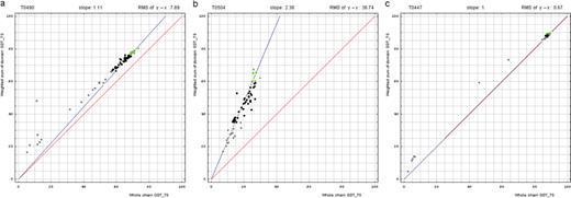
Correlation between domain-based evaluation (y, vertical axis) and whole-chain GDT-TS (x, horizontal axis). (a) A typical correlation plot for target T0490. (b) A plot of target T0504 showing beneficial domain evaluation for this target. (c) A plot of target T0447 showing unnecessary domain evaluation for this target. Each point represents first server models. Green, gray and black points represent the top 10, the bottom 25% and the remaining prediction models, respectively. The blue line is the best-fit slope (intersection 0) to the top 10 server models. The red line is the diagonal. The slope and RMS y − x distance for the top 10 models (average difference between the weighted sum of domain GDT-TS scores and the whole-chain GDT-TS score) are shown above the plot.

The points lie above the diagonal. Apparently, the weighted sum of domain predictions is higher than the whole-chain GDT-TS for this example. This difference results from a domain arrangement that is a bit different between target and template. Thus, while individual domains are modeled well, their assembly is predicted worse. We measure the difference between the weighted sum and the whole-chain GDT-TS by two parameters: root mean square (RMS) and slope. The RMS difference between the weighted sum of GDT-TS on domains and GDT-TS on the whole chain (RMS of y − x) measures absolute GDT-TS difference. A slope of best-fit line with intercept set to 0 (slope) measures relative GDT-TS difference. These parameters are computed on top 10 (according to the weighted sum) predictions.

The target on the plot (T0490) is a four-domain protein. The slope and the RMS of y − x are 1.1 and 7.8, respectively. Do these parameters justify splitting the target into four domains and using them individually in the combined evaluation of predictions? To answer this question, we examined correlation plots for all targets.

Here, we illustrate two extreme examples. First, for T0504, which is a triplication (three domains) of an SH3-like barrel, the plot revealed that while individual domains are predicted reasonably well (Figure 1b): domain GDT-TS above 60 for some servers, their inter domain packing was not: whole-chain GDT-TS about 20. The whole-chain score is three times less than the weighted sum over three domains, indicating that the domain arrangement was modeled randomly by servers and did not closely match the target domain arrangement. Obviously, domain evaluation is beneficial for this target. Second, for T0447, which is also a three-domain target, the plot revealed that the weighted sum and the whole-chain GDT-TS are about the same, clustering near 90% GDT-TS for all template-based servers (Figure 1c). Clearly, domain-based evaluation for this target is not different from whole-chain evaluation and does not reveal any interesting prediction features.

Before we examine all targets to find a data-dictated cutoff for domain-based evaluation, an additional issue needs to be addressed. Some proteins, while being evolutionarily single-domain proteins, experience domain swaps. Such swaps are defined as a structural ‘exchange’ of protein regions between monomers in an oligomer. For instance, T0459 is a dimeric winged Helix-Turn-Helix (wHTH) domain with an N-terminal β-hairpin (blue). This N-terminal β-hairpin (blue) packs against a different chain (white), and a β-hairpin (white) from the other chain packs against the first chain (rainbow), illustrating the swap (Figure 2a). A rainbow-colored compact domain composed of segments from both chains of the swap is illustrated in Figure 2b.

Figure 2.

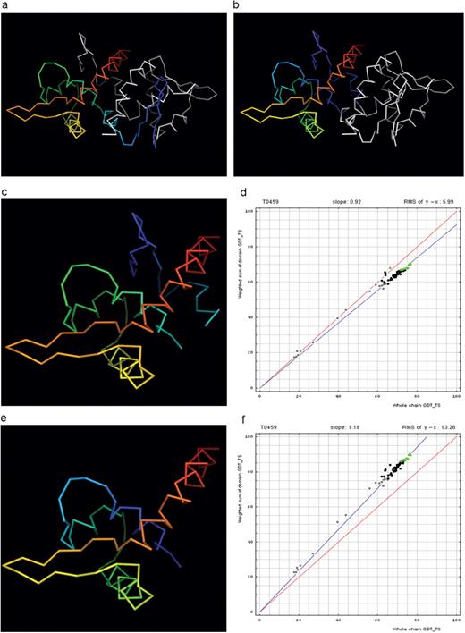
Domain swap example (a) T0459 chain A (rainbow) with its symmetry mate (white). (b) T0459 chain A with a swapped N-terminal β-hairpin from its symmetry mate chain (rainbow) and the swapped hairpin symmetry mate chain (white). (c) Domain-swapped T0459 with chain B: 2–22 plus chain A: 23–106. (d) Correlation between GDT-TS scores for T0459 domain-based evaluation with a swapped domain (y, vertical axis) and whole-chain GDT-TS (x, horizontal axis). (e) T0459 with domain-swapped segment removed: chain A: 23–106. (f) Correlation between GDT-TS scores for T0459 domain-based evaluation with N-terminal segment removed (just A: 23–106, y, vertical axis) and whole-chain GDT-TS (x, horizontal axis).

Since predictions correspond to monomers, swapped models do not appear globular (i.e. Figure 2a, blue). However, some servers may somewhat correctly predict the globular swapped monomer (i.e. Figure 2b, rainbow). Alternatively, servers may not predict either of the two positions for the swapped region, and evaluation over the domain core with the swapped region removed can be useful. Considering these alternatives, three evaluations were performed on targets with domain swaps. For instance, we used three structures in T0459 evaluation: whole chain, swapped domain (Figure 2c) and domain with swapped segment removed (Figure 2e). Correlation plots for the two domain definitions (swapped and swapped segment removed) of this single-domain target reveal differences (Figure 2d and f).

For single-domain targets, the y-axis shows the GDT-TS for domain evaluation, as the weighted sum is computed over a single domain. The points falling below the diagonal in Figure 2d (swapped domain) indicate that servers missed the swap, placing the N-terminal hairpin closer to its position in a whole (although less globular) chain. As expected, the points fall above the diagonal in Figure 2f, as the difficult-to-predict region was removed from the target. From these plots, however, the usefulness of either of these domain-based evaluations compared with the whole-chain evaluation remains unclear.

To find a cutoff for using ‘domain-based’ versus ‘whole-chain’ evaluation, we analyzed the correlation of the RMS of the difference between domain GDT-TS and whole chain GDT-TS (RMS of y − x) and the slope of the 0 intercept best-fit line (slope) for all targets (Figure 3).

Figure 3.

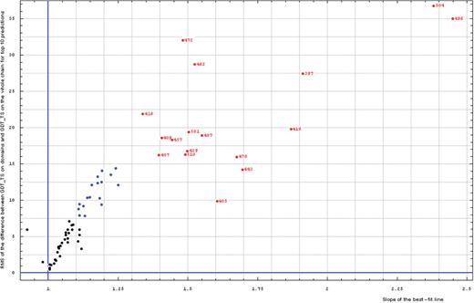
Correlation between RMS of the difference between GDT-TS on domains and GDT-TS on the whole chain (vertical axis) and the slope of the best-fit line (horizontal axis), both computed on top 10 server predictions.

Most targets cluster in the region for RMS of y − x below 15 and slope below 1.3, representing similar domain-based evaluation and whole-chain evaluations (black and blue points). Clearly, a few targets (red points, target numbers shown for each point) exhibit large differences and should be evaluated by domains separately. The targets with intermediate properties (blue points, RMS of y − x above 7.5) fall within the natural trend of the black points and do not stand out in obvious ways.

In summary, comparison of domain-based predictions with whole-chain predictions revealed a natural, data-dictated cutoff (slope of the zero intercept best-fit line is above 1.3) to select targets that require domain-based evaluation. These targets are: T0397, T0407, T0409, T0416, T0419, T0429, T0443, T0457, T0462, T0472, T0478, T0487, T0496, T0501, T0504 and T0510. Predictions for other targets follow the general trend of showing a more similar quality for ‘domain’ and ‘whole chain’ indicating that domain-based evaluation may not be necessary. This cutoff corresponds particularly to CASP8 targets and predictions, and may not translate other target/prediction sets. Accordingly, blindly applying a 1.3 slope cutoff to other data sets without performing similar analysis should be avoided.

To combine target scores, we limited individual domain analysis to ‘red’ targets in evaluation tables. All other targets were evaluated as whole chain in domain-based evaluation tables: they are considered to be single-domain targets for the purpose of CASP8 evaluation. However, all domain-based evaluation results for all targets are shown on individual target pages and are available for analysis and model visualization. These ‘domains’ include single domain proteins with certain structure regions removed, and swapped domains.

Target categories

Some targets are easy to predict, having very close templates among known structures, while other targets are quite challenging. Since the performance of different algorithms depends on target difficulty, taking this characterization into account becomes essential for evaluating predictions. Grouping targets into categories of approximately the same prediction difficulty brings out the flavors of how each method deals with different target types.

In the early days of CASP, targets were classified and evaluated in three general categories: comparative modeling, fold recognition and ab initio prediction, to reflect the method used to obtain models (1, 19). It became clear with time that the best approach to fold prediction is to use a combination of these various methods, as what matters is the quality of the final prediction. Therefore, an alternate grouping of targets into categories based on the prediction quality is logical.

A general approach described here leads to well-defined category boundaries determined naturally from the data. The approach is rooted in a suggestion by the Baker group to use prediction scores of the top 10 models (see ROBETTA evaluation pages http://robetta.bakerlab.org/CASP8_eval/) and is similar to what we used for target classification in the CASP5 assessment (20). We resorted to a traditional model quality metric that stood the test of time—LGA (18) GDT-TS scores. Targets for which domain-based evaluation is essential were split, while other targets remained as whole chains (see above discussion). This procedure resulted in 147 ‘domains’ gathered from 125 targets. For each of these domains, the top 10 GDT-TS scores for the first server models were averaged and used as a measure of each target's difficulty.

We looked for naturally emerging clusters in these average GDT-TS scores using a density-based algorithm. The Gaussian kernel density estimator (8) is

where n is the number of domains, μ_i is average GDT-TS score for a domain i, and σ is a standard deviation, called bandwidth. Conceptually, each domain score generates a Gaussian centered at that score with standard deviation σ. Averaging of these Gaussians gives a density function ρ(x) that reveals score groups. The maxima of this function correspond to group centers, and the minima mark the boundaries between groups. When the bandwidth is very narrow (= variance very small), each domain forms its own group. When the bandwidth is broad (= variance very large), all domains form one group. Some optimal bandwidth setting should reveal meaningful groups in the data.

We plotted estimated densities for varying bandwidths, from 0.3 to 8.2 GDT-TS% units (Figure 4). Apparently, the lower end bandwidth (0.3%) is too small and results in too many clusters (magenta curves on a plot below). Alternatively, higher bandwidths around 8% (cyan curves) reveal only two major groups: a large cluster centered at about 73% GDT-TS and a smaller one around 41%. These major clusters can be used for evaluation, as they demonstrate the data set splitting naturally into ‘hard’ and ‘easy’. A surprisingly nonsurprising cutoff (52% GDT-TS) defines the boundary between these two groups. A bandwidth of 4% (black curve) yields three groups traditionally analyzed by CASP: hard (AI), medium (FR) and easy (CM) (52 and 81% cutoffs, respectively). The ‘medium’ group splits the former ‘easy’ group of the two-cluster breakdown. Finally, a 2% bandwidth (yellow-framed brown curve) reveals five groups, and this is about the right number for evaluation of predictions. GDT-TS boundaries between these groups are 30, 52, 68 and 81%. We term these categories: FM (as predictors are free to do anything, yet they still fail to predict these targets right), FR (to give a tribute to a historic category) and CM_H, CM_M and CM_E. We use these categories to evaluate server predictions. Whole chain prediction analysis revealed identical trends, with the same cutoffs of 30, 52, 68 and 81% used to determine the target category from the top 10 averaged first model GDT-TS scores.

Figure 4.

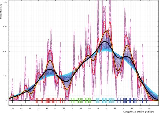
Gaussian kernel density estimation of domain GDT-TS scores for the first model GDT-TS averaged over top 10 servers and plotted at various bandwidths (= standard deviations). These average GDT-TS scores for all domains are shown as a spectrum along the horizontal axis: each bar represents a domain. The bars are colored according to the category suggested by this analysis: black, FM; red, FR; green, CM_H; cyan, CM_M; blue, CM_E. The family of curves with varying bandwidth is shown. Bandwidth varies from 0.3 to 8.2 GDT-TS% units with a step of 0.1, which corresponds to the color ramp from magenta through blue to cyan. Thicker curves: red, yellow-framed brown and black correspond to bandwidths 1, 2 and 4, respectively.

Scores and evaluation

Having a good score to evaluate predictions is crucial for method development. Many approaches are trained to produce models scoring better according to some evaluation method. Thus, flaws in the evaluation method will result in better scoring models not representing real protein structures in any better way. One such emerging danger is compression of prediction model coordinates, which decreases the gyration radius and may increase some scores that are based on Cartesian superpositions. Assessment of predictions by experts, as done in CASP, is essential to detect such problems (21).

Nevertheless, a good automatic approach that mimics expert judgment is desirable. For CASP5 predictions, we found (20) that the average of Z-scores computed on sever model samples for many different scoring systems correlates best with expert, manual assessment. These scoring systems should represent different concepts of measuring similarity, such as Cartesian superpositions, intramolecular distances and sequence alignments. Among various suggested scores, GTD–TS computed by the LGA program (18) represents the best as a single score to reflect the model quality. This reflection is probably because GTD–TS ombines four scores, each computed on a different superposition (1, 2, 4, and 8 Å). However, GTD–TS scales with the gyration radius and is influenced by compression. We analyzed server predictions using three scoring systems: the classic LGA GTD–TS, and two novel scores designed to address model compression. Superimpose the model with the target using LGA in the sequence-dependent mode, maximizing the number of aligned residue pairs within d = 1, 2, 4, and 8 Å.

1. As a cornerstone of this evaluation, we computed GTD–TS scores for all server models using the LGA program. This score represents a standard in the field, it is always shown first, and score tables are sorted by it by default. We call this score TS, i.e. ‘total score’, for short.

2. The GTD–TS score measures the fraction of residues in a model within a certain distance from the same residues in the structure after a superposition. This approach bases on a ‘reward’ concept. Each residue placed in a model close to its ‘real’ position in the structure is rewarded, and the reward depends on the proximity of that modeled residue. As an analogy with physical forces, such a score accounts for only the ‘attraction’ part of a potential and ignores any ‘repulsion’ component. The ‘reward’-only concept might have been reasonable in the past, when predictions were quite poor, and detecting any positive feature of a mainly negative model was the key. Today, many models accurately reflect experimental structures. When the positives start to outweigh the negatives, paying attention to the negatives becomes important (22). Thus, we introduced a ‘repulsion’ component into the GDT-TS score that penalizes a residue that is too close to ‘incorrect’ residues (other than the residue that is modeled). This idea was suggested by David Baker as a part of our collaboration on CASP and model improvement. We refer to this new score as TR, i.e. ‘the repulsion’. The TR score rewards close superposition of corresponding model and target residues while it penalizes close placement of other residues. This score is calculated as follows.

For each aligned residue pair, calculate a GDT-TS-like score: S₀(R₁, R₂) = 1/4 [N(1) + N(2) + N(4) + N(8)], where N(r) is the number of superimposed residue pairs with the CA–CA distance < r Å.

Consider individual aligned residues in both structures. For each residue R, choose residues in the other structure that are spatially close to R, excluding the residue aligned with R and its immediate neighbors in the chain. Count numbers of such residues with CA–CA distance to R within cutoffs of 1, 2, and 4 Å. (As opposed to GDT-TS, we do not use the cutoff of 8 Å as too inclusive.)

The average of these counts defines the penalty assigned to a given residue R: P(R) = 1/3 * [N(1) + N(2) + N(4)]

Finally, for each aligned residue pair (R₁, R₂), the average of penalties for each residue P(R₁, R₂) = 1/2 * (P(R₁) + P(R₂)) is weighted and subtracted from the GDT-TS score for this pair. The final score is prohibited from being negative:

Among tested values of weight w, we found that w = 1.0 produced the scores that were most consistent with the evaluation of model abnormalities by human experts. We studied the correlation between the GDT-TS and two new scores: TR and CS. For each domain, the top 10 scores for the first server models were averaged and used to represent a score for a domain. These averages are plotted for TS and TR scores (Figure 5a). TS and TR scores are well correlated, with Pearson correlation coefficient equal to 0.991. Since TR is TS minus a penalty, TR is always lower than TS. Moreover, the trend curve of the correlation is concave, hence TR scores are more different from TS scores around the mid-range, where models become less similar to structures and modeled residues are frequently placed too close to the nonequivalent residues resulting in a higher penalty. For very low model quality (TS below 30%) rewards are relatively low, so penalties also drop. TS and CS scores are also correlated (Pearson correlation coefficient is 0.969), but to a less extent than TS and TR scores (Figure 5b). Nevertheless, this correlation is very good considering the differences in scoring methods: TS is based on superpostions, but CS is a superposition-independent contact-based score.

1. Scores comparing intramolecular distances between a model and a structure (contact scores) have different properties than intermolecular distance scores based on optimal superposition. One advantage of such scores is that superpositions, and thus arguments about their optimality, are not involved. Contact matrix scores are used by one of the best structure similarity search program DALI (23). The problems with developing a good a contact score are (i) contact definition; (ii) mathematical expressions converting distance differences to scores. In our procedure, contact between residues is defined by a distance ≤ 8.44 Å between their C_α atoms. The difference between such distances in a model and a structure is computed and used as a fraction of the distance in the structure. Fractional distances above 1 (distance difference above the distance itself) are discarded and the exponential is used to convert distances to scores (0→1). The factor in the exponent is chosen to maximize the correlation between contact scores and GDT-TS scores. These residue pair scores are averaged over all pairs of contacting residues. We call this score CS, i.e. ‘contact score’, for short. It should not be confused with a general abbreviation for a ‘column score’ used in sequence alignments.

Figure 5.

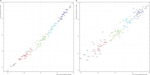
(a) Correlation between TR score (vertical axis) and GDT-TS (horizontal axis). (b) Correlation between contact score CS (vertical axis) and GDT-TS (horizontal axis). Scores for top 10 first server models were averaged for each domain shown by its number positioned at a point with the coordinates equal to these averaged scores. Domain numbers are colored according to the difficulty category suggested by our analysis: black, FM (free modeling); red, FR (fold recognition); green, CM_H (comparative modeling: hard); cyan, CM_M (comparative modeling: medium); blue, CM_E (comparative modeling: easy).

In addition to using reasonable scores, tabulating evaluations requires a model for random comparison. The model we use takes a target structure into account. We modify the target structure by circularly permuting it and shifting (threading) a sequence along the chain with a step of five residues. That is, for a target of n residues, amino acid 1 is placed at the site 6, 2 at the site 7, i [1 ≤ i ≤ (n − 5)] at the site i + 5, and n − j (0 ≤ j < 5) at the site 5 − j. For a chain of n residues, [integer part of (n/5) − 1] such modified structures are made.

Each of these modified structures is compared with the original structure to compute a score. Since the coordinates of the structure are not modified in this process and only the sequence is assigned to given coordinates differently, our procedure does not give a meaningful random comparison for all types of scores, e.g. DALI Z would be highly elevated for a random score if computed on this model. However, the GDT-TS, TR and CS scores we use in our evaluation behave as expected, and this ‘permutation-shift’ random model works well for them.

Additionally, we increase the number and diversity of these random comparisons by considering a ‘reverse chain’ model, when the sequence is threaded onto the structure from C- to N-terminus and sequence shifts along the chain are made. More specifically, amino acid 1 is placed at the site n, 2 at the site n − 1, and i at the site n − i + 1. This procedure forms one of the ‘random’ structures. Then shifts with permutations are made to it as described above and we obtain [integer part of n/5] structures (Figure 6).

Figure 6.

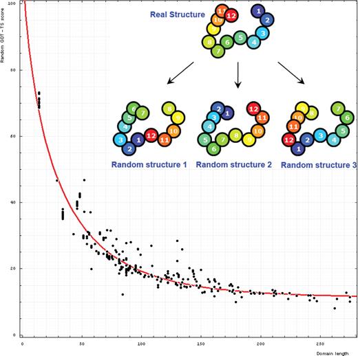
Dependence of GDT-TS (vertical axis) on domain length (horizontal axis). Each point represents a random score for a domain. All NMR models for each domain are used, and random scores for them appear as vertical streaks giving an idea about random errors of random scores. The red curve is the best-fit of the function mentioned in the text. On the upper right, one example indicates the procedure generating random structures. Random structure 1: permuted and residue 1 is placed at position 6 of the original structure; random structure 2: reverse chain and random structure 3: reverse chain, permuted and residue 1 is placed at position 6 of the reverse chain structure.

Random scores show strong reverse correlation with length (Figure 6). Random GDT-TS scores can be well-fitted with a function a Exp(b Length^c) − a Exp(b 2^c) + 100, where the best-fit parameter values are a = 102.814, b = 0.089 and c = 0.729. This function is designed to give a random score of 100 for Length = 2, i.e. for a protein of two residues any random superposition will lead to a perfect match. For Length → ∞, the random score approaches a value larger than 0. Using the following function one can estimate the random GDT-TS score for a domain of ‘Length’ residues:

In addition to giving a reference point for prediction of difficult targets, these random scores are utilized when a server does not provide a model for a particular target. Difficulties arise in computing a sum of scores for all targets for a given server in cases where some scores are negative or missing. If a certain type of score can only be positive, missing predictions contribute a reasonable 0 to the total score. However, for Z-scores, poor predictions get negative scores. In this case a server not submitting predictions for some targets (score 0) will do better than a server submitting less than average predictions (negative Z-scores). Omitting all negative scores from summation, as has been done in former years of assessment, provides one solution for this discrepancy. However, with improved quality of models, negative Z-scores should probably penalize a server. Thus, we include negative scores in summation and replace missing models with random computed Z-scores. So, not submitting a prediction is equivalent to submitting a ‘random’ prediction in our assessment.

Interestingly, some servers submitted predictions of inferior quality to that of random predictions. Although this observation seems a bit counterintuitive, it makes sense when the model is inspected. Such worse-than-random predictions are much less compact than real proteins. A random protein, with similar secondary structure composition and length to the target, will result in better score than a nonprotein-like model.

Since the details of predictions are discussed in the official CASP8 assessment and in the publications by predictors (including Baker-Grishin group), they are not elaborated upon in this work. Our database allows for each prediction model to be interactively visualized in PyMOL. As a main general observation, human groups provided better predictions than automatic servers. The first server (Zhang-Server) ranked fifth using GDT-TS scores combined over all targets; the next best server (ROBETTA) ranked 22nd. This improved performance by human groups reflects, at least in part, the availability of all server models to ‘human’ predictors. Human groups were allowed about 3 weeks to generate a target, while servers were allowed only 3 days, with their predictions openly accessible after submission. Some human groups (i.e. Zhang group) operated as ‘meta-predictors’ by automatically combining server predictions to produce the best model. With this strategy, Zhang ranked second by GDT-TS scores. Only a few human groups actually utilized expert knowledge on protein structures and did not benefit from the availability of server predictions. Among these, not mentioning the DBAKER group, the most notable was Ceslovas Venclovas (IBT_LT group).

Interesting targets

New folds

‘New folds’ was a prominent category in early CASPs. Now, defining it as a ‘category’ is hardly possible. New folds are rapidly approaching extinction. In fact, the majority of structure types may already be known for water-soluble proteins. We agree with the result from the Skolnick group (24) that structure space knowledge is close to complete as far as distinct types of secondary structure packing are concerned. However, this statement is very far from saying that we know how to map sequence space on structure space. The deduction of many folds from sequence is currently not possible, as confirmed by CASP8 results. Many families with ‘old’ folds are not predictable from sequence. For instance, no server found the correct template for T0460, and confident predictions were not possible for T0465, T0466, etc. Thus, structural biologists still have a long road ahead as structural genomics reveals and will continue to find many wonderful examples of unusual occurrences of such sequence-unpredictable ‘old’ folds hiding among the semi-random families being structurally characterized.

By new folds we mean distinct cores of secondary structural elements with connections and spatial arrangement not observed before. Although fold definition is subject to debate, experts frequently agree on what looks like a ‘new fold’. Several experts in our group inspected CASP8 target structures and concluded that only two domains represent new folds: T0397_1 and T0496_1.

Nevertheless, some similarities exist between each of these domains and existing PDB structures. The N-domain of T0397 (T0397_1, Figure 7a) displays some topological resemblance to a Ferredoxin-like fold (Figure 7b), with a curved β-sheet and α-helices deteriorated into loops. The ferredoxin-like core is elaborated with a loop and a β-strand (green) inserted into its β-hairpin and a β-strand (red) at its C-terminus. N-domain of T0496 (Figure 7c) shares similarity with an RNAseH fold (Figure 7d), and may even be viewed as a circular permutation of it.

Figure 7.

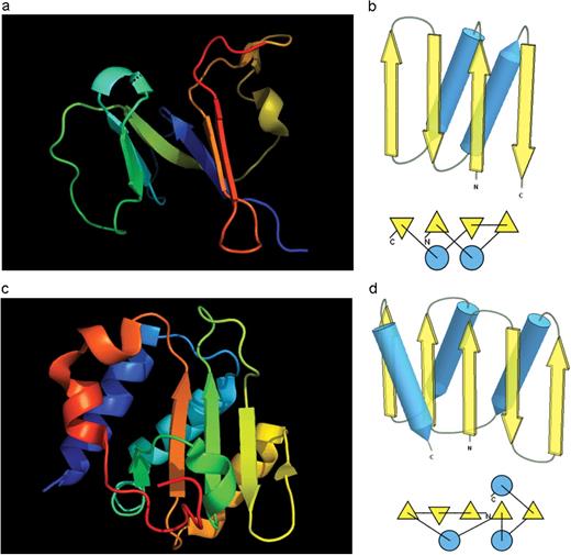
(a) Cartoon diagram of N-terminal domain of T0397: 3d4r chain A residues 7–82. (b) Structure and topology diagrams of ferredoxin fold–fold closest to T0397 N-terminal domain. (c) Ribbon diagram of N-terminal domain of T0496: 3d09 chain A, residues 4–126. (d) Structure and topology diagrams of RNAseH fold–fold closest to T0496  N domain.

Server predictions for both of these new folds were quite poor. However, our analysis shows that two other targets, clearly with known folds, i.e. T0407_2: an IG-like domain; and T0465: a FYSH domain (5), were also predicted very poorly. Apparently, as far as structure prediction is concerned, little difference exists between new folds and known folds for which templates are not detectable from sequence. Due to this observation and the relatively small number of new folds, CASP category definition should be based on a different criterion, e.g. quality of a few best server predictions.

Evolutionary analysis of unusual CASP8 proteins

T0467

In our opinion, this target represents the most interesting CASP8 example, because it unexpectedly revealed a segment of likely analogous (not homologous) sequence similarity found by servers. While this segment is good for modeling the structure locally, extension of the alignment to cover the entire domain results in a wrong fold prediction.

T0467 represents an OB-fold, which is a five-stranded β-barrel, in this instance partly open between the 3rd and the 5th β-strands (Figure 8a1). This fold similarity is not detectable at statistically significant levels by known sequence methods. The first COMPASS (25) hit to an OB-fold protein is to the SCOP Nucleic acid-binding domain superfamily, ranked #24 in the total list of hits with an insignificant E-value around 25. Moreover, SH3 domain proteins, which form a five-stranded β-barrel, were found by COMPASS prior to this hit. Nevertheless, nine consensus match residues in the COMPASS alignment map to structurally equivalent positions validating the OB-fold hit and suggesting a possible evolutionary relationship with Nucleic acid-binding domains.

Figure 8.

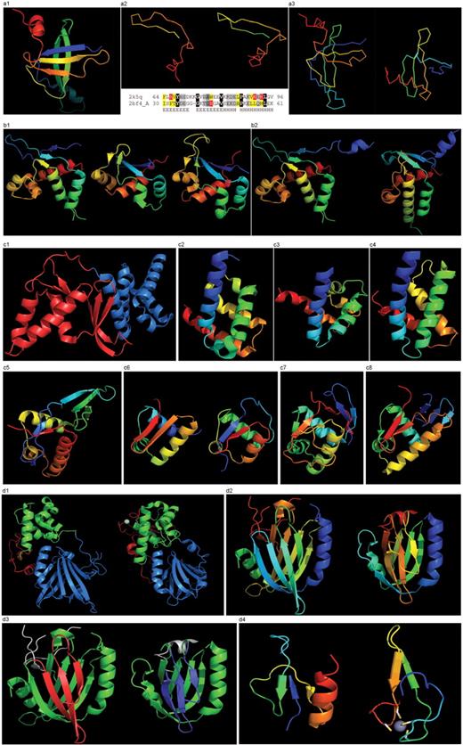
(a1) Cartoon diagram of T0467: 2k5q model 1, residues 7–97. (a2) Ribbon diagram of T0467 OB-fold C-terminal terminal region and Sso7d SH3-fold C-terminal region. Left: T0467 OB-fold C-terminal fragment: 2k5q model 1, residues 64–97; Right: Sso7d SH3-fold C-terminal fragment: 2bf4 chain A residues 30–64. On the bottom of this panel, a sequence alignment between 2k5q and 2bf4 indicates the sequence similarity between OB-fold and SH3-fold. (a3) Ribbon diagram of T0467 global OB-fold and Sso7d global SH3-fold. Left: T0467 OB-fold: 2k5q model 1, residues 7–97; Right: Sso7d SH3-fold: 2bf4 chain A. (b1) Cartoon diagram of T0465 and two typical proteins with FYSH domain. Left: Cartoon diagram of T0465, 3dfd chain A residues 21–136; Middle: FYSH domain of hypothetical protein AF0491: 1t95 chain A residues 11–94; Right: FYSH domain of hypothetical protein Yhr087W: 1nyn chain A residues 1–93. (b2) Cartoon diagram of T0465 and the closest template 2bo9. Left: Cartoon diagram of T0465: 3dfd chain A residues 11–137; Right: bacteriophage HK97 tail assembly chaperone: 2ob9 chain A. (c1) Cartoon diagram of T0443 evolutionary domains: 3dee, N- and C-terminal domains are colored blue and red, respectively. (c2) Cartoon diagram of N-terminal domain of T0443: 3dee residues 31–117. (c3) Middle domain of eIFα: 2aho chain B residues 96–176 belongs to SAM-domain fold. (c4) Four helices from a cyclin domain: 1gh6 chain B 648-733. (c5) Cartoon diagram of C-terminal domain of T0443: 3dee residues 118–230, HTH helices are orange-yellow and orange, ‘wing’ strands are blue and red (c6) Left: classic-winged HTH in biotin repressor: 1bia residues 1–63, HTH helices are green and yellow, ‘wing’ strands are orange and red; Right: circularly permuted HTH in Met aminopeptidase: 1b6a 378-446, HTH helices are yellow and orange, ‘wing’ strands are blue and red. (c7) 2nd HTH in cullin: 1ldj chains A:586–673, B:19–28, HTH helices are green and lime, ‘wing’ strands are yellow and orange, side β-sheet is red and blue. (c8) HTH domain of PhoB: 1qqi residues 10–104, HTH helices are green and yellow-orange, ‘wing’ strands are orange and red, side β-sheet is blue-cyan. (d1) Left: cartoon diagram of T0510 domains: 3doa, N-terminal, middle and C-domains are shown in blue, green and red, respectively; Right: cartoon diagram of MutM domains: 1ee8_A, N-terminal, middle and C-terminal domains are shown in blue, green and red, respectively, Zn ion is shown as a white ball. (d2) Left: N-terminal domain of 510: 3doa residues 1–165; Right: N-terminal domain of MutM: 1ee8 chain A residues 1–121. (d3) Left: N-terminal domain of 510: 3doa residues 1–165 insertion close to the N-terminus is red; Right: N-terminal domain of MutM: 1ee8 chain A residues 1–121 insertion in the middle of the domain is blue. (d4) Left: N-terminal domain of 510: 3doa residues 236–279; Right: N-terminal domain of MutM: 1ee8 chain A residues 230–266.

This OB-fold was predicted de novo by ROSETTA (26), which correctly indicated an open barrel. This prediction was very suggestive of the correct structure, because ROSETTA is biased towards local β-strand pairing, and the OB-fold has a crossing loop to form H-bonds between β-strands 1 and 4, not to mention the barrel closure present in most OB-folds with H-bonds between β-strands 3 and 5. The metaserver bioinfo.pl (27) fails to find similarity to other OB-fold proteins, and incorrectly provides SH3-like predictions. Although some servers used OB-folds as templates, the significance of those predictions is unclear as the templates were closed barrels. Many servers used SH3-fold templates or closed OB-fold templates. The bias towards an SH3 fold is likely caused by the C-terminal region, which shows strong local conformational similarity to Sso7d Chromo-domain DNA-binding proteins (28).

This similarity covers about 30 residues (half of Sso7d SH3-fold) and spans through a β-hairpin and two α-helices (Figure 8 a2). The first helix is a single-turn helix characteristic of the SH3 fold. Such a helix, frequently structured as a 3₁₀-helix, is present at this spatial location in the majority of SH3-fold proteins. Mutual orientations of four secondary structural elements between the two fragments (from OB and SH3) are very similar, as reflected by sequence similarity of alignments. Server detection of this similarity is not surprising. However, upon closer inspection several positions with charged residues (highlighted red in the above alignment) align to hydrophobic residues (yellow). These positions display different exposure to solvent in the two structures and hint that the local similarity may not translate to the global fold similarity. Indeed, the two C-terminal helices form essential core elements in the SH3 structure of Sso7d, but are peripheral surface helices not in the OB-fold of T0467. In addition, the surface of the hairpin buried in the SH3-fold is exposed in T0467. These inconsistencies in hydrophobic patterns are very suggestive of global structural differences (Figure 8 a3).

DALI-LITE (23) does not detect this local similarity, but aligns the central three-stranded meander β-sheet in the two proteins (shown in the back on the images Figure 8 a3: blue-cyan-green in T0467, and green-yellow in Sso7d), albeit with a very low Z-score of 0.3 (33 residues, RMSD 2 Å). This globally meaningful Dali alignment (only residues in capital letters are aligned) superimposes hydrophobic cores of both proteins.

As a summary, superposition of locally similar fragments in SH3- and OB-folds does not result in global superpositions of structural cores, and does not result in a reasonable fold prediction. Vice versa, global superposition of the cores leaves the two locally similar fragments as nonequivalent parts of the two proteins, as they occupy very different spatial locations and carry out different structural roles.

Global similarity between OB- and SH3-folds has been noticed previously (29), and explained in terms of very distant evolutionary relationship (homology). The 20-folds could share a common ancestor, being homologous over the three-stranded curved meander sheet, although definitive evidence for this presumption is lacking. The meaning of the local fragment similarity between T0467 and Sso7d-like chromo-domain OB-fold proteins is unclear. These similar fragments could have originated independently with their conformational resemblance due to chance, thus representing a rare example of analogous sequence similarity.

T0465

As opposed to T0467, extension over the entire domain of a short, 30-residue alignment results in a correct fold prediction for this target. As weak HHsearch (30) and COMPASS (25) hits suggest, and 3D structure confirms, this example is a mildly distorted FYSH domain (5). HHsearch aligns T0465 with FYSH domain protein as the first hit, but with rather low probability (∼24%). COMPASS also finds this alignment as the 17th hit with an E-value of ∼20. An N-terminal β-hairpin (blue-cyan) is followed by α-hairpin (cyan-green) and a short β-strand to complete the sheet (lime-yellow). The next β-strand typical of a FYSH domain is missing in T0465. Two C-terminal α-helices of FYSH (orange-red) are replaced with three α-helices in T0465 (Figure 8 b1). Thre bacteriophage HK97 tail assembly chaperone 2ob9 would be the closest structure to T0465 (Figure 8 b2); however, no server found it as a template.

T0443

This is an unusual protein from a large family (Figure 8 c1). The N-terminal domain represents a SAM-domain (HhH motif) fold (31), with both HhH motifs deteriorated. The loops typically housing the motifs are still possibly functional for DNA binding (Figure 8 c2 and c3). Additionally, DALI (23) finds partial, but quite significant (Z-score > 5) similarity to the cyclin fold, matching four out of five cyclin helices. If detected by any server, this template would produce a very accurate starting model (Figure 8 c4). The C-terminal domain represents a circularly permuted wHTH, i.e. the last strand of the ‘wing’ is the first strand of the domain, like in methionine aminopeptidase (Figure 8 c5 and c6).

Additionally, the winged HTH in the C-domain is decorated with a three-stranded sheet inserted after the ‘wing’. β-hairpins and strands are known to be present just before the N-helix of the three-helical HTH domains, e.g. cullin 1st HTH (Figure 8 c7) and PhoB-like domains (32) (Figure 8 c8). The HTH conformation looks a bit unusual, probably due to strong crystal contacts that bend the α-helices. The molecule is probably a dimer that binds a small ligand with two conserved Arg residues (one is not even modeled in the structure, it is just N-terminal to the first modeled residue), each from each monomer. This protein family is very large, and a similar kind of HTH without the N-domain exists as a separate protein: ‘Coenzyme PQQ synthesis protein D’. Interestingly, The HHpred server (33) finds HTH domains (e.g. 2dql) as templates for this C-terminal domain. The first COMPASS hit in the SCOP database is to the DNA/RNA-binding three-helical bundle HTH-containing superfamily. Although the E-value estimate is only marginally significant (∼0.4), the alignment is largely correct and can be used for template-based modeling of the C-domain.

T0510

This target has three domains, with a dramatic structural change in the N-terminal domain belonging to the MutM-like DNA repair proteins N-domain fold (34), and a less striking, but nevertheless significant change in the C-terminal domain, which is a deteriorated treble-clef finger with a Glucocorticoid receptor-like (DNA-binding domain) fold (35). The middle domain was the easiest to predict as it kept the conserved S13-like H2TH fold.

The N- and C-terminal domains of T0510 experience amazing structural transformations compared with the homologous protein MutM (34) (Figure 8 d1). T0510 and MutM are homologous throughout the chain in all three domains, retaining similar relative positioning of these domains. However, a closer look at the N-terminal domains reveals large topological differences (Figure 8  d2). Although the architecture appears similar between the two proteins: two β-sheets flanked on the sides by two α-helices, the topology is quite different. The β-sheet facing the viewer is N-terminal (blue-cyan-green) in T0510, and is inserted in the middle of the molecule (yellow-orange) in MutM. Common superimposable parts of both molecules are shown in green below, with different insertions colored red and blue (Figure 8 d3). T0510 has a three-stranded insertion (red) after the N-terminal α-helix, and MutM has a three-stranded insertion (blue) after the 4th common β-strand. Although both insertions form three-stranded antiparallel β-sheets, they are different in topology: a meander in T0510, and a βLββ in MutM. Insertions are not surprising in remote homologs. However, convergence to similar architecture through independent insertions/deletions is not very common.

Despite this interesting peculiarity, there is no doubt about the homology between N-domains of these proteins. COMPASS being queried with just the N-terminal domain sequence, without a more similar H2TH middle domain, finds the first MutM protein as the 16th hit. The COMPASS alignment is correct in the middle region. The C-terminal domain in T0510 is a treble-clef finger that lost its Zn-binding site, has deteriorated beyond recognition and has gained the C-terminal β/α-unit (Figure 8 d4).

Acknowledgements

We would like to thank David Baker and the members of his group, in particular J. Thompson, S. Raman, R. Vernon, E. Kellogg, M.D Tyka, O. Lange, D.E. Kim and R. Das for many insightful discussions during our work on CASP8 predictions; CASP organizers John Moult, Krzysztof Fidelis, Andriy Kryshtafovych, Burkhard Rost and Anna Tramontano for their vision, leadership and discussions during the CASP8 meeting in Italy; structural biologists, in particular PSI consortia, who generously provided structures for CASP8; and predictors who developed servers that generated predictions making this work possible. This work was supported in part by NIH grant GM67165 and Welch foundation grant I1505 to NVG.

Conflict of interest. none declared.